 Sign in
 Anonymous
on June 12th 2014
0
Anonymous
on June 12th 2014
0
Ordinary Bézier curve is a special case or rational Bézier curve
should be
Ordinary Bézier curve is a special case of rational Bézier curve
 | What is a NURBS?April 6th 2006 |
This article explains the term NURBS, describes basic properties of NURBS curves and surfaces, and gives examples how they are used in 3D modeling.
To understand this article you should have basic knowledge about vector and 3D graphics.
Curves are found in various areas of computer graphics. They are used when creating 3D models, vector images, animations, or for example in definition of TrueType fonts. There is a great variety of curves. Some are easy to use, some are flexible enough to describe a large variety of shapes, and some are simple enough to be implemented and accelerated by graphics hardware.
NURBS and Bézier curves are ones of the most commonly used curves and the focus of this article.
Before explaining NURBS, we will stop by Bézier curve, because NURBS is a generalization of Bézier curve. The following figure shows a simple Bézier curve (C), its control points (1), (2), (3), (4), and its control polygon (P). The control points are also called control handles.

A cubic Bézier arc (C) with its control polygon (P).
Each point on a Bézier curve (and on many other kinds of curves) is computed as a weighted sum of all control points. This means that each point is influenced by every control point. The first control point has maximum impact on the beginning of the curve, the second one reaches its maximum in the first half of the curve, etc.
Each control point influences the final curve according to assigned blending function. A blending function defines the weight of the control point at each point of the curve. A value of 0 indicates that the control point is not affecting a point on the curve. If the blending function reaches 1, the curve is (usually) intersecting the control point.

Blending functions of a cubic Bézier curve.
Four functions for four control points - each in different shade of red.
Properties of blending functions define properties of a curve. Bézier curves use polynomial functions of given degree. The resulting curves have these properties:
The previous example showed a cubic (degree 3) curve, which is one of the most often used types. The degree refers to the highest exponent in the polynomial blending functions used for Bézier curves. A Bézier curve may be of arbitrary degree. A degree 1 curve is a simple line and has two control points. A degree 2 curve is an arc and has three control points. The higher the degree, the more control points and the more complex shape is possible. But it is also more much harder to use, because each control point still influences the whole curve.
Each control point in rational curve is assigned a weight. The weight defines how much does a point "attract" the curve. Only the relative weights of the control points are important, not their absolute values. A curve with all weights set to 1 will have the same shape as if all weights are set to 100. The shape only changes if weights of control points are different.
Ordinary Bézier curve is a special case of rational Bézier curve, where all weights are equal. Rational curve gives designers additional options at the cost of a more complicated algorithm and additional data to keep track of.
A B-Spline consists of multiple Bézier arcs and provides an unified mechanism how to define continuity in the joins.
Consider two cubic Bézier curves - that is 8 total control points (4 per curve).

B-Splines consist of Bézier arcs.
Lets make the last point of the first (green) curve equal to the first point of the second (violet) curve - this saves us 1 point leaving us with 7 total control points. We have replaced one control point with an external condition.
The third (blue) curve and the fourth (yellow) curve share ending points just like in previous case, but they also have the same tangent direction at the junction point. There are two external conditions and only 6 control points are necessary to describe the curves.
B-Splines use external conditions to put multiple pieces together while keeping the original concept of control points. The neighbor curves share some control points. External conditions are either implicit (uniform curves) or explicitly given by a knot vector. Knot vector defines how much information should be shared by neighbor curves (segments).
Knot vector is a sequence of numbers, usually from 0 to 1, for example (0, 0.5, 0.5, 0.7, 1), and it holds the information about external conditions mentioned earlier. Number of intervals defines number of segments (3 in our case: 0-0.5, 0.5-0.7, 0.7-1). Numbers in knot vector are called knots and each knot has its multiplicity. Multiplicity of knot 0.7 is 1, while multiplicity of knot 0.5 is 2. The higher the multiplicity, the less information share the neighbor segments. When multiplicity is equal to the degree of used curves, there is a sharp edge (green and violet curves on the image).
NURBS stands for Non-Uniform Rational B-Spline. It means NURBS uses rational Bézier curves and an non-uniform explicitly given knot vector. Therefore, degree, control points, weights, and knot vector are needed to specify a NURBS curve.
So far, we were talking about curves - one-dimensional formations. The principles can be applied to higher-dimensional objects like surfaces or volumes. Surfaces are used when creating 3D objects, for example landscapes while volumes can be used to define a non-linear transformation.
Following screenshots demonstrate different uses of NURBS in 3D graphics.
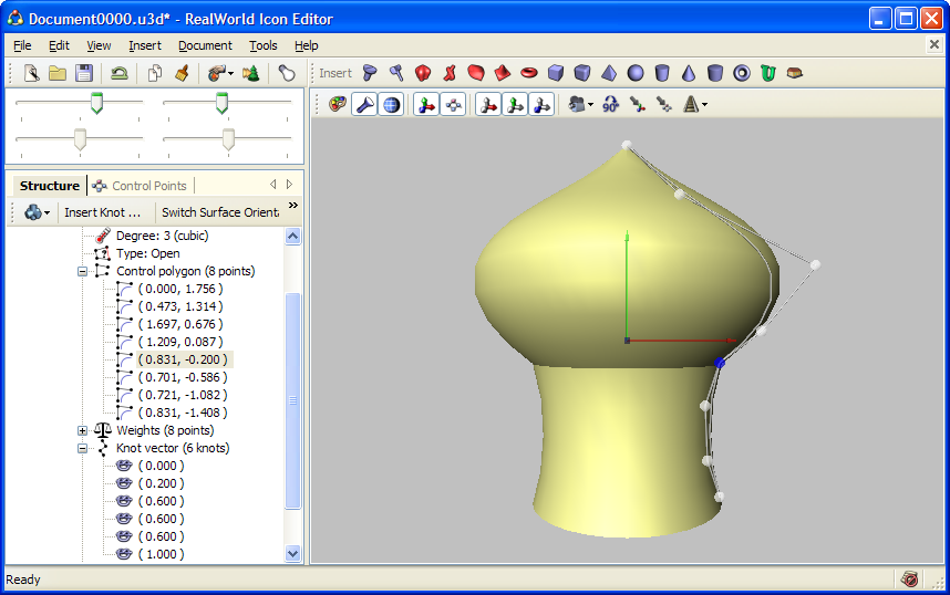 Surfaces or revolution can roughly approximate relatively large amount of different shapes. | 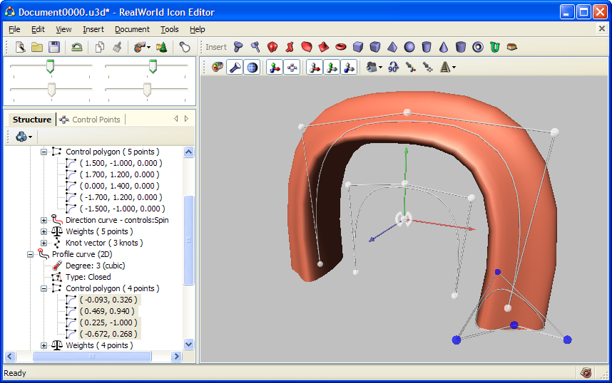 Surface was created by moving a 2D NURBS curve along a path defined by another 3D NURBS curve. |
The left image demonstrates a surface created by revolving a 2D NURBS curve around Y axis. The curve itself consists of 3 pieces (knot vector: 0, 0.2, 0.6, 0.6, 0.6, 1). Join between the two upper pieces is smooth, because the multiplicity of knot 0.2 is 1 and curve degree is 3. On the other hand, knot 0.6 with multiplicity 3 causes a sharp edge.
The right image shows a surface created by sweeping a 2D curve along a 3D trajectory.
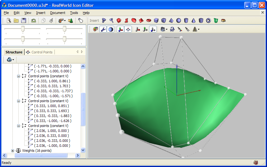 NURBS surfaces need relatively large amount of control points, which makes them hard to control. | 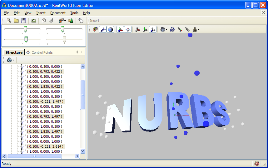 The middle part of the text is magnified and the text is bent using a 2nd degree NURBS volume. |
Left image shows a NURBS surface and its control points. NURBS surfaces are used rather rarely in their pure form because the number of control points is usually large (4x4 in our simple case) and the surface becomes hard to control.
Right image shows a 3D text that was transformed using a Bézier (or NURBS) volume of degree 2. The text is bent and its central part is larger - that effect was caused by the non-linear transformation defined by the NURBS volume (note the control points in the center of the model).
When working with NURBS in their pure form, there is one very useful operation: inserting new knot. A knot can be inserted into a NURBS curve without changing the shape of the curve. The desired side effect of this operation is an additional control point that provides finer control of the related region of the NURBS curve or surface.
There are other operations with NURBS, like elevating degree, removing knots, or computing control point positions from points laying on a curve, but they do not reach the usefulness of knot insertion.
This article described the fundamentals of NURBS from user's point of view by demonstrating their properties on simple examples.
While NURBS curves are relatively simple and anyone can learn to effectively use them after a bit of practice, NURBS surfaces are much harder due to the large amount of control points. Therefore many applications offer various methods that simplify and limit their capabilities.
The problematic of curves in computer graphics is much larger than this introductory article indicates; readers are advised to seek other sources of information and to gain first hand experience.
 Recent commentsAnonymous
on June 12th 2014
0
Recent commentsAnonymous
on June 12th 2014
0
Ordinary Bézier curve is a special case or rational Bézier curve
should be
Ordinary Bézier curve is a special case of rational Bézier curve
Anonymous
on September 4th 2014
0
so if i am drawing a 2D drawing off of a print and i want to use nurbs how do figure the weight for each point. is there a formula?
If you drawing manually, you should probably not bother with weights, leave them all the same. You can approximate shapes with various accuracies in multiple ways.
Anonymous
on August 22nd 2017
0
Thanks 😮
Anonymous
on December 8th 2018
0
podrian poner el nombre de la persona que escribe el articulo, eso seria aun mas genial
😊
Anonymous
on June 15th 2021
0
我看不懂,但是大受震撼
Anonymous
on June 15th 2021
0
can't understand
Anonymous
on October 7th 2021
0
Great step through and example based education of curvy, curby, nerdy NURBS.
ok
Nurbs are hard to make for me.

 reddit
 Facebook share